Aug 10, 2024
Quantitative Analysis of Bitcoin Transaction Feerate
A formula can be very simple, and create a universe of bottomless complexity.
---Benoit Mandelbrot
Overview
Any user can submit a transaction to modify the shared state of the Bitcoin network. A decentralized network of full nodes with limited resources provides settlement assurance for transactions. Due to the inelastic supply of blockspace, users engage in competition for the allocation of finite computational capacity through a transaction fee mechanism.
This study seeks to deepen the understanding of Bitcoin transaction fee dynamics through quantitative analyses, focusing on two primary aspects: establishing statistically robust and model-free bounds for Bitcoin feerate, and investigating the volatility clustering effect using historical data.
As a coda, we demonstrate that integrating these analyses can serve as a basis for modeling future ranges, offering a framework for predicting future Bitcoin feerate and pricing financial instruments linked to Bitcoin feerate. We will publish updated results using these methods on an ongoing basis.
Bounds Analysis
To begin, we will attempt to establish statistically robust upper and lower bounds for the feerate index. For simplicity, we will take the median Sat/vB of the transactions in each block, and take the average across the observation period.
Given an observation period of length l days, we define a ratio R(t,l,q):
MovingAverage(t,q) is the function to calculate the moving average of an index at time t with q days of averaging.
q is the moving average lookback window, (e.g. q=1 means spot rate and q=7 means weekly average).
This ratio essentially measures how much the index's average across the observation period changes from the moving average at the start of the period.
We employ a non-parametric approach to calculate the bounds for ratio R based on historical data. This method is advantageous for its replicability and its departure from traditional parametric techniques, which may not accurately capture complex market dynamics.
The objective is to ensure that the probability of the ratio 𝑅 exceeding these bounds is de minimis. The derivation of the bounds involves three key steps:
Recent percentile-based bounds Define the bounds initially to be at least the $xth $percentile of the realized ratio, R, over the preceding n days. This premise is grounded in the notion that the index's recent performance is reflective of current market conditions. For example, we set x=0.99 (99th percentile) and n=180 days.
Incorporating delta change Historical data reveals a negative correlation between the magnitude of R and its delta change within certain time intervals. In other words, the smaller the R is, the larger its change. To accommodate this, the upper bound includes an additional buffer based on the discrete delta change of R over the preceding n days.
To avoid overfitting, we segment the historical data into s equally sized groups over the same n-day window. We then calculate the xth percentile of R's delta changes, conditional on the segmented sample.
Constraint by longitudinal historical performances The upper bound is further restrained by the xth percentile of R over a longer span, here we are using five years.
Given an index with a realized ratio Rt,l,q, the upper bound UBt,l,k and lower bound LBt,l,k for an observation period of length l, with k days forward starting window, at current time t, are determined by the following expressions:
where:
m=min(R) over 5 years.
s=4(quartile);
f(Rl,t,n,s,y,k) is a function to find yth percentile of the ratio Rl’s l+k days delta change conditional on sampling with the group that is evenly divided into s that level of Rt−l−k,l falls into from the last n days.
Using an observation period of 15 days with a 3-day forward starting window, we backtest the historical data from 1/1/2018 to 07/31/2024 and derived the following bounds:

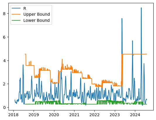
Moreover, the consistent xth percentile threshold across the three steps can be derived and used by setting a goal of coverage rate, for example, 90% or 95%. We will publish the bounds on a weekly basis on our Substack. Subscribe here.
Indicative pricing within bounds
We have established statistically robust upper and lower bounds for the feerate index with fixed observation periods. With bounds calibrated such that the probability of average feerate falling out of bounds is smaller than a predefined threshold. Next, we propose a model-independent way to provide indicative pricing based on the bounds.
We calculate the expected value of a function of the ratio R (as explained in the previous section) from all historical data, where the function bounds the ratio R with a given Alkimiya Pool parameters.
For example, there are 3 pools for 15-day BTC fee contracts from Aug 1st to Aug 15th, 2024, with floor - cap of 1.0 - 13.0 Sat/vB, 13.1 - 30 Sat/vB, and 31 - 55 Sat/vB, respectively. In this case, the ratio R is defined as the latest 15-day average feerate divided by the 15-day average 15 days ago without any forward starting. At the end of July 2024, the latest 15 day average feerate is 5.14 Sat/vB, the calculation shows that there are 93.85%, 4.80% and 0.72% probabilities that the realized average feerate will fall into the three buckets respectively. The expected value of feerate pricings based on the ratio R and latest 15 day average feerate are 5.6, 13.4 and 31.1 Sat/vB respectively. Note that the pricings for the two pools with higher cap and floor are very close to the floors. This is because a low chance of realization might cause capital inefficiency on the seller side, given higher collateral requirements. The seller is selling out-of-money options, which collect the premium if the options expire worthless.

Volatility Clustering
The feerate market exhibits dynamic self-adjustment in response to fluctuations in blockspace demand. In this section, we use time series analyses to calculate the model-dependent pricing expectation for different pools. We examine the presence of volatility clustering in Bitcoin transaction fees.
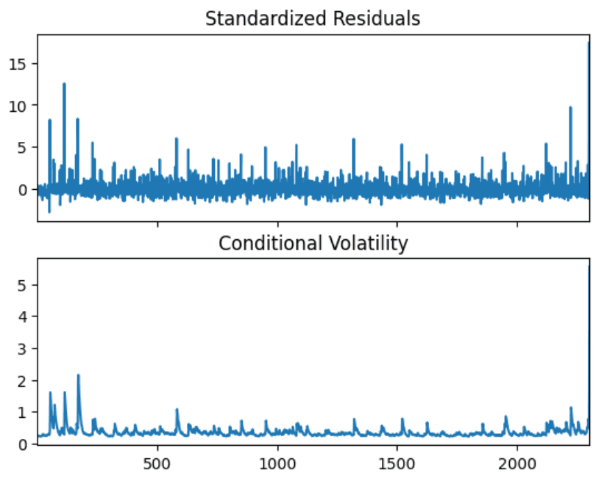
Volatility clustering describes the phenomenon where periods of heightened or reduced volatility tend to occur in succession, akin to the behavior observed in seismic activity, where clusters of rapid and intense events follow extended periods of quiescence. This indicates that periods of significant (or minimal) changes in transaction fees are likely to be followed by similarly significant (or minimal) changes, rather than random fluctuations.
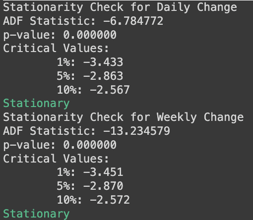
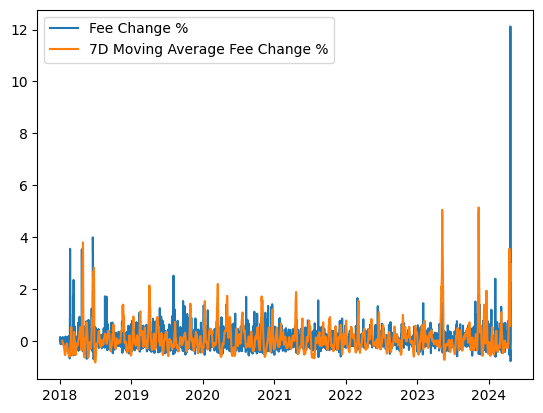
Before applying time series modeling techniques, it is necessary to ensure the data set is stationary. A stationary time series typically results in improved model performance. The constancy of key statistical properties ensures that models can better capture the underlying dynamics, leading to more accurate predictions. Typical methods to convert a time series into a stationary one include differencing, detrending, removing seasonality, and so on. For financial time series analysis, daily percentage change and weekly percentage change of the 7-day moving average are two candidates for stationarity purposes. Both time series on Bitcoin transaction fees pass the stationarity test (augmented Dickey-Fuller test).
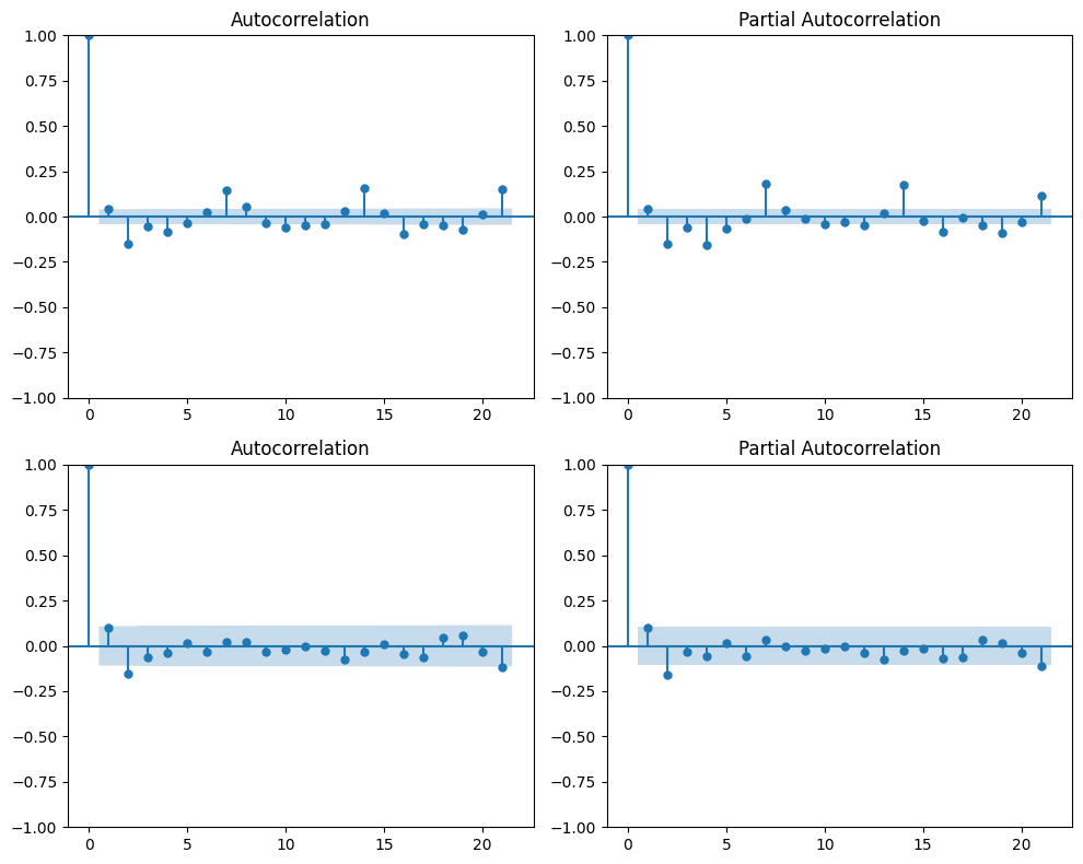
The ACF and PACF plots of daily and weekly change data suggest that autoregressive–moving-average (ARMA) models can be applied to both series, given the autocorrelation and partial autocorrelation behavior of the Bitcoin feerate data.
Notably, the (partial) autocorrelations demonstrate seasonality on a weekly scale, suggesting that a SARIMA (Seasonal Autoregressive Integrated Moving Average) model might be preferred. For instance, a SARIMA(p,d,q)×(P,1,Q)7 model yields comparable results by differencing the weekly data.
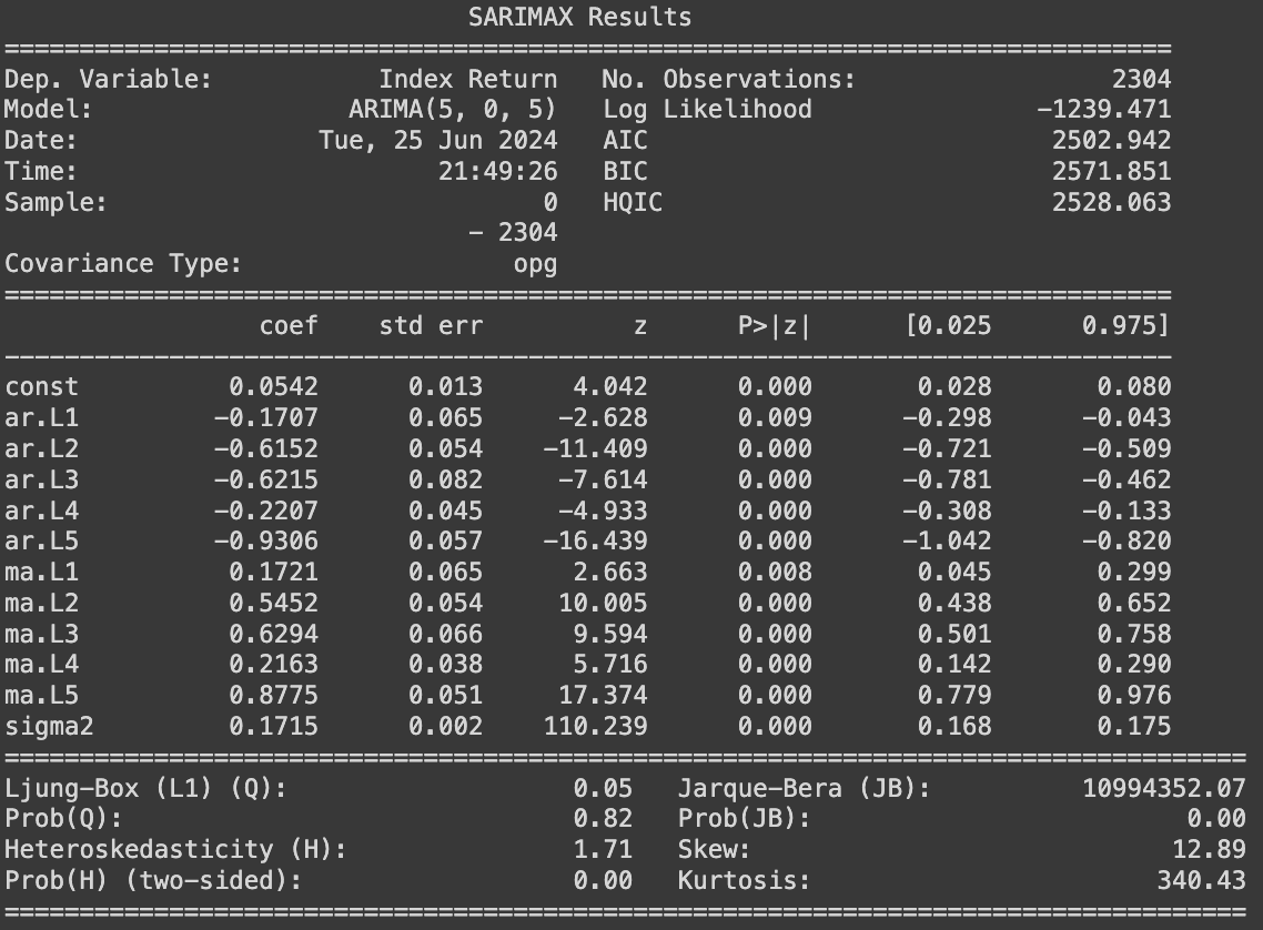
On the daily return data, the $ARIMA(5,0,5) $model performed well from 2018, which might help to predict the expected (narrow) range of the data in the future with the data points from last week. However, the variance of the error terms is not constant across time; hence, it is impossible to predict the movement accurately when variance/volatility changes over time.
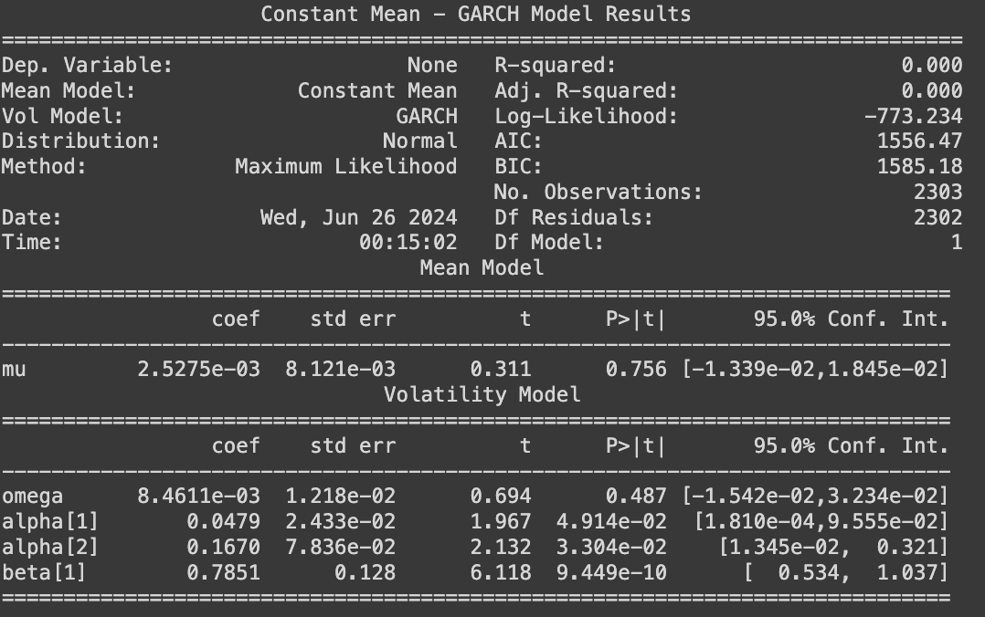
A generalized autoregressive conditional heteroskedasticity (GARCH) model can be deployed to analyze the variance evolution. GARCH models were created in the context of econometric and finance problems having to do with the amount that investments or stocks increase (or decrease) per time period, so there’s a tendency to describe them as models for that type of variable. The model uses values of the past squared observations and past variances to model the variance at time t. Please note that ARIMA and GARCH models can be trained from Maximum Likelihood Estimate (MLE) sequentially or simultaneously.
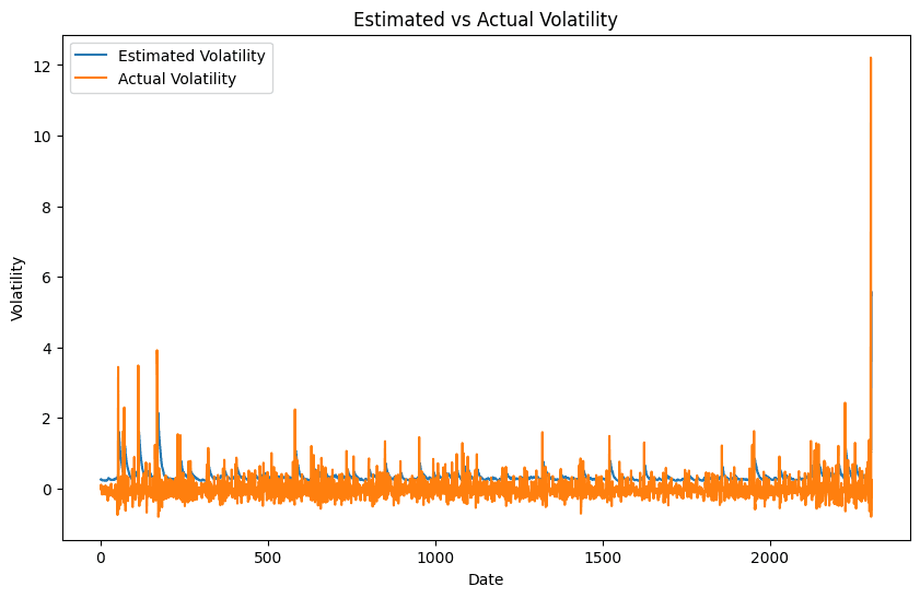
In this research piece, a sequential GARCH(2,1) model fits well with the residuals from the ARIMA(5,0,5) on daily return data, which suggest that the volatility of bitcoin transaction fee change depends on the past residuals and volatility for previous days, i.e., the volatility clustering is presence. Hence ARIMA(5,0,5)−GARCH(2,1) can be deployed to analyze and predict the expected range for future fee.
Weekly Return Data
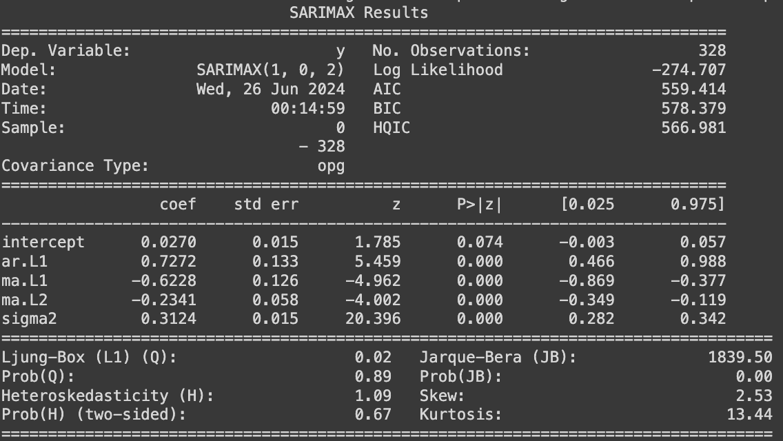
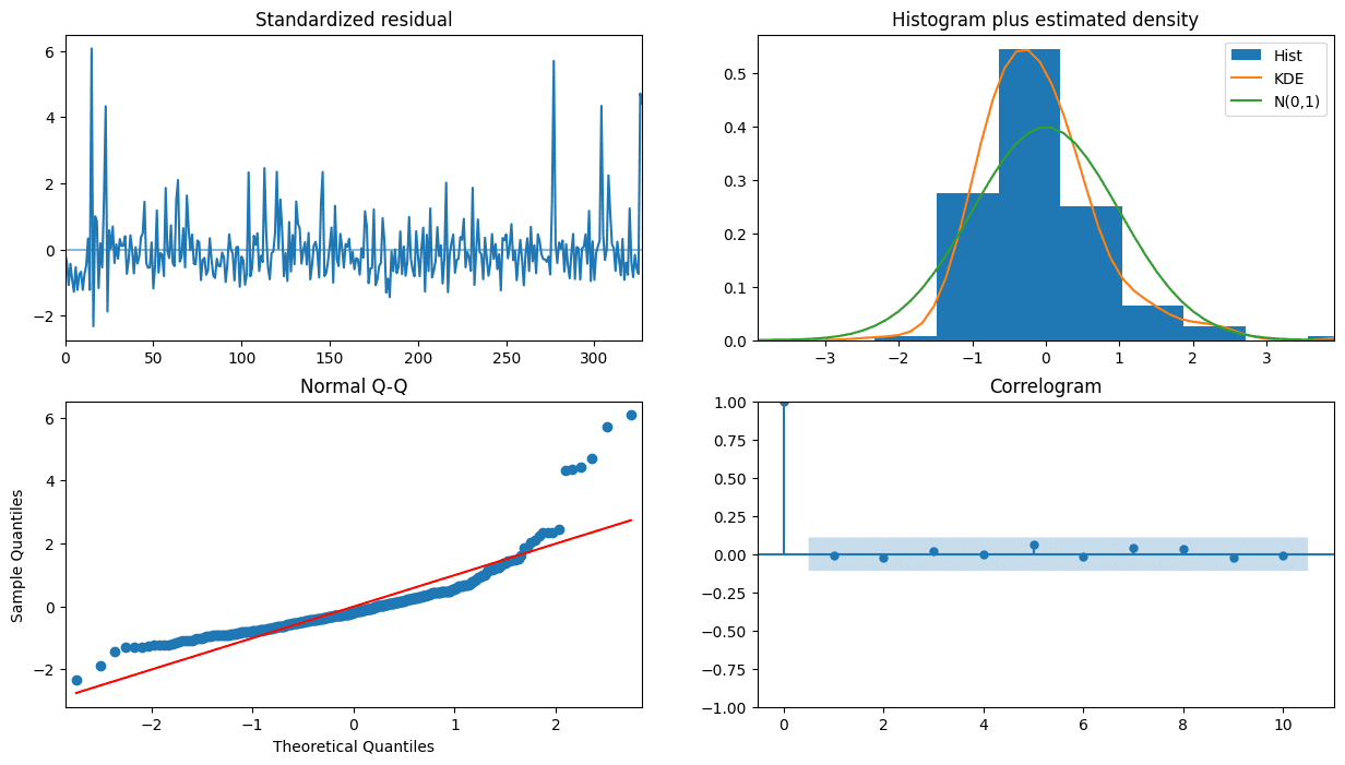
Looking at weekly return data, ACF and PACF plots of weekly sampling data show significant autocorrelations at lags 1 and 2. After parameter tuning, an $ARIMA(1,0,2) $model preserves the relationship while maintaining the model simplicity (based on AIC and BIC metrics). The time series model incorporates one autoregressive and two moving-average terms to regulate the stationary stochastic process and determine the expected value of future data points.
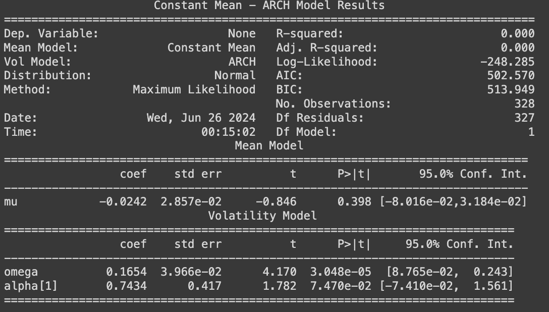
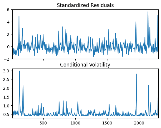
Similar to the daily sampling, variance can be better explained by a stochastic or time-dependent process. A sequential GARCH(1,0) model (effectively an ARCH(1) model) fits well with the residuals from the ARIMA(1,0,2) on weekly return data, suggesting the presence of volatility clustering on a weekly level, especially with lag 1. Hence ARIMA(1,0,2)−GARCH(1,0) can be deployed to analyze and predict the expected range for the following week’s transaction fee to some degree with a confidence interval.
An ARIMA(p,d,q)−GARCH(P,Q) model can provide users with an educated estimate of fee spikes in the next period based on historical data within a confidence interval. However, when persistent volatility clustering is present, the model's performance may be limited. Therefore, financial instruments for hedging exposure might be preferable for those concerned about spiking transaction costs. Please note that ARIMA(p,d,q)−GARCH(P,Q) model can be applied to determine the bounds (in the previous section) for a short period of future given recent fee data, however, the results are highly model dependent. In contrast, a model-independent bounds mechanism is preferred for generalization purposes.

The presence of volatility clustering is helpful in determining how much premium to bake into feerate contracts. When the volatility clustering effect is observed, it is expected that contracts should price in a greater premium, given the higher chance of drastic movements. We will also publish updated results on an ongoing basis.
Conclusion
Public blockchains have a finite capacity for blockspace resources, and therefore, all on-chain actions compete for inclusions and orderings with transaction fees. While scaling solutions can reduce the amount of full-node resources consumed per operation, pricing the right to access them real-time is a fundamentally market-based challenge at a global scale.
By establishing statically robust bounds and examining the presence of volatility clustering, we offer a framework that combines non-parametric approach and well-fit models for predicting and pricing future feerates.
Future research could investigate alternative stochastic volatility models, such as the Merton Jump-Diffusion model combined with the Heston model, where the variance process varies according to the square root of variance. Comparing these models with time series approaches could provide comprehensive insights.
